Understanding The Convolutional Layer in State Space Models
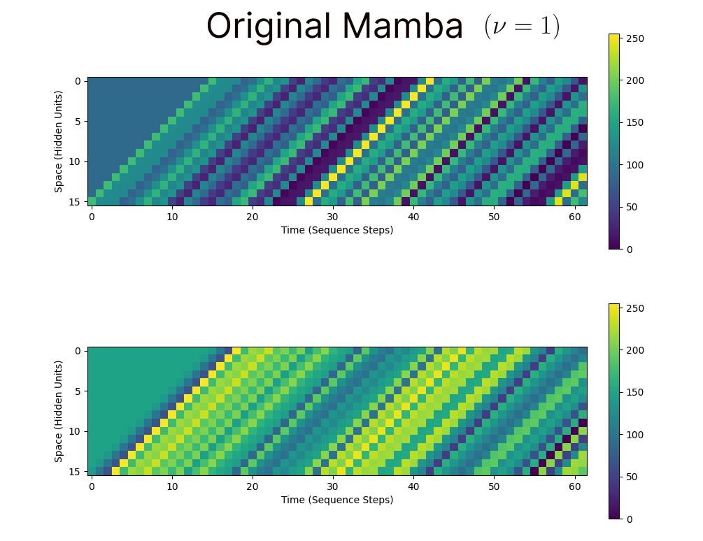
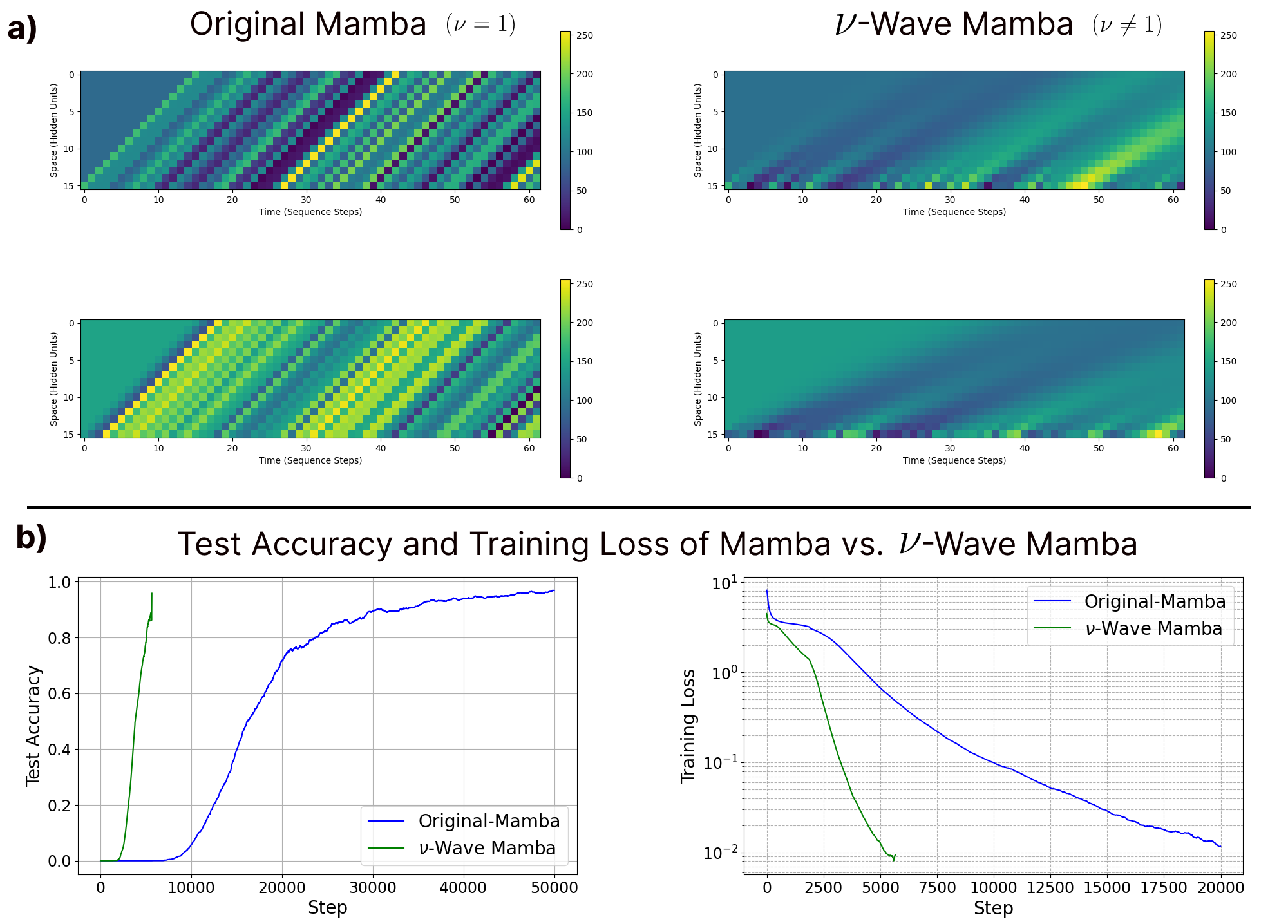 Visualization of traveling waves found in the original Mamba architecture (left) and the variable velocity traveling waves we introduce in the Nu-Wave Mamba model (left). We see the variable velocity model learns exponentially faster and reaches lower error than the original counterpart.
State Space Models (SSMs) such as Mamba, Griffin, and xLSTM have recently approached the language modeling performance of Transformer architectures such as GPT and Llama. Interestingly, these models all share a common peculiar core component of their ‘block’ structure – a specific small convolutional kernel applied over the time dimension. In this blog post, we will aim to answer the question: Why is this particular architectural motif conserved across so many state of the art models? To do so, we will revisit the origin of this convolutional layer, tracing it back to one of the first SSM blocks built specifically for language, the Hungry Hungry Hippos (H3) block. We will aim to return emphasis to the original interpretation of this layer as a ‘Shift-SSM’, and highlight how the reformulation as a convolutional layer obscures its underlying computational purpose while simultaneously harmfully restricting the possible parameterizations of the model. As a means to better understand the fundamental role of this now widely adopted layer, we will show how the Shift-SSM is related to a recent class of recurrent neural networks which aim to introduce ‘traveling waves’ of activity in their hidden state as a form of memory. We will provide a true ‘Shift-SSM’ implementation of Mamba, allowing for the visualization of these waves and experimentation with a full parameterization. Ultimately, we present this post as a helpful guide on the purpose and origin of the now widely adopted convolutional layer in modern SSMs, hoping to reveal a path to improvements of such models.
T. Anderson Keller
Conference Abstract: https://akandykeller.github.io/papers/NuWaveMamba.pdf
Introduction
In recent years, a class of recurrent neural network models have risen in popularity as a potential alternative to the ubiquitous Transformer architecture. A number of such recurrnet models have now been built, often falling under the umbrella-term of ‘State Space Models’ (SSMs). Their appeal is largely derived from their similar scaling capability as Transformers, granted by efficient algorithms for processing linear recurrences in a way that is sub-linear in computation time with respect to sequence length. Furthermore, given that they are inherently recurrent models, they also admit faster test-time inference complexity, allowing for substantial speed-ups in deployment after training.
In this post, we will focus on a few of the recent architectures built primarily for language modeling, which have been shown to approach the state of the art performance of large pretrained Transformer models. Particularly, we will focus on a specific architectural motif, namely a small 4-element convolutional kernel applied over the sequence length, which has been conserved across all of these models without much explanation. In this post, we will explain in detail how this component can be better understood by its original interpretation as an SSM with a specific shift-operator recurrence. We provide what we believe to be the first implementation of an actual Shift-SSM within an SSM ‘block’, highlighting the additional tunable parameters that are only realized in this framework, and otherwise held-fixed at specific pre-determined values when treated jointly as a convolution. We will further extend this parameterization by showing a direct relation with a recent class of recurrent neural networks based on traveling wave dynamics, visualizing the waves which thereby already propagate through existing SSMs, and suggesting a many new paths for improving such models in the future.
State Space Model Background
State Space Models are most commonly introducted with the following differential equations: \[\begin{aligned} \mathbf{\dot{x}}(t) & = \mathbf{A}\mathbf{x}(t) + \mathbf{B}u(t), \\ y(t) & = \mathbf{C}\mathbf{x}(t) + \mathbf{D}u(t), \end{aligned}\]
where \(\mathbf{x}(t) \in \mathbb{R}^N\) is the state vector, \(u(t) \in \mathbb{R}^1\) is the time-dependant input signal, \(\mathbf{A} \in \mathbb{R}^{N \times N}\) is the recurrent connectivity matrix, \(\mathbf{B} \in \mathbb{R}^{N \times 1}\) maps from the input to the hidden state, \(\mathbf{C} \in \mathbb{R}^{1 \times N}\) maps from the hidden state to the target signal \(y(t) \in \mathbb{R}^1\). Most work asserts that \(\mathbf{D} \in \mathbb{R}^{1 \times 1}\) is set to \(0\) (and we will also follow this convention in this post), but it can equivalently be viewed as a skip-conection.
These continuous-time equations are then often discretized with a specific timestep size \(\Delta\), through what is known as a Zero-Order-Hold method (ZOH), which approximates the input signal \(u(t)\) as constant between timesteps \(t\) and \(t + \Delta\). This yields the following discrete recurrence, \[\begin{aligned} \mathbf{x}_{k} & = \mathbf{\bar{A}}\mathbf{x}_{k-1} + \mathbf{\bar{B}}u_k, \\ y_k & = \mathbf{\bar{C}}\mathbf{x}_k + \mathbf{\bar{D}} u_k, \end{aligned}\]
where \(\mathbf{x}_{-1} = \mathbf{0}\), \(\mathbf{\bar{A}} = \mathrm{exp}(\Delta \mathbf{A})\), \(\mathbf{\bar{B}} = (\mathrm{exp}(\Delta \mathbf{A}) - I) (\Delta \mathbf{A})^{-1} \Delta \mathbf{B}\), and \(\mathbf{C}\) & \(\mathbf{D}\) remain unchanged (i.e., \(\bar{\mathbf{C}} = \mathbf{C}\), \(\bar{\mathbf{D}} = \mathbf{D}\)). This is an exact numerical integration of the continuous time equations, assuming the approximation of the input signal is correct (Jacquot, 2019).
Acceleration through Global Convolution
The above equations can be seen to represent a Linear Time Invariant (LTI) system, and they have a long history of study in the control theory literature. Early work in the SSM community leveraged the linearity of the operations in this recurrence to efficiently accelerate computation by effectively pre-computing the associated operators for each timestep, converting the full recurrence into a single global convolution. This convolution can then be efficiently accelerated by performing the operation in Fourier space. Explicitly, letting \(\mathbf{x}_{-1} = \mathbf{0}\) the convolutional form can be derived by seeing that the value of \(y\) at each timestep can be computed by unrolling the recurrence: \[\begin{aligned} y_0 & = \mathbf{\bar{C}} \mathbf{\bar{A}}\mathbf{x}_{-1} + \mathbf{\bar{C}}\mathbf{\bar{B}}u_0,\\ & = \mathbf{\bar{C}}\mathbf{\bar{B}} u_0, \\ y_1 & = \mathbf{\bar{C}} \mathbf{\bar{A}}\mathbf{x}_{0} + \mathbf{\bar{C}}\mathbf{\bar{B}}u_1, \\ & = \mathbf{\bar{C}} \mathbf{\bar{A}}\mathbf{\bar{B}}u_0 + \mathbf{\bar{C}}\mathbf{\bar{B}}u_1,\\ y_2 & = \mathbf{\bar{C}} \mathbf{\bar{A}}\mathbf{x}_{1} + \mathbf{\bar{C}}\mathbf{\bar{B}}u_2,\\ & = \mathbf{\bar{C}} \mathbf{\bar{A}}(\mathbf{x}_{0} + \mathbf{\bar{A}}\mathbf{\bar{B}} u_0) + \mathbf{\bar{C}}\mathbf{\bar{B}}u_2,\\ & = \mathbf{\bar{C}} \mathbf{\bar{A}}^2\mathbf{\bar{B}} u_0 + \mathbf{\bar{C}}\mathbf{\bar{A}}\mathbf{\bar{B}}u_1 + \mathbf{\bar{C}}\mathbf{\bar{B}}u_2,\\ \vdots & \\ y_k & = \mathbf{\bar{C}} \mathbf{\bar{A}}^k\mathbf{\bar{B}} u_0 + \mathbf{\bar{C}} \mathbf{\bar{A}}^{k-1}\mathbf{\bar{B}} u_1 + \dots + \mathbf{\bar{C}} \mathbf{\bar{A}}^{0}\mathbf{\bar{B}} u_k, \\ & = \left[\mathbf{\bar{C}} \mathbf{\bar{A}}^k \mathbf{\bar{B}},\ \mathbf{\bar{C}} \mathbf{\bar{A}}^{k-1} \mathbf{\bar{B}}\ \ldots\ \mathbf{\bar{C}} \mathbf{\bar{A}}^{0} \mathbf{\bar{B}} \right] \cdot \left[u_0,\ u_1,\ \ldots\ u_k\right]. \end{aligned}\]
Thus, the entire output sequence \(\mathbf{y}\) can be computed as: \[\begin{equation*} \mathbf{y} = \mathbf{\bar{K}} \star \mathbf{u} \end{equation*}\]
where \(\mathbf{\bar{K}} = \left(\mathbf{\bar{C}} \mathbf{\bar{A}}^i \mathbf{\bar{B}} \right)_{i=0}^L\) is the associated convolutional kernel, applied over the entire length \(L\) sequence \(\mathbf{u} = [u_0, u_1, \ldots u_L]\). Note that this convolutional kernel has the same size as the entire sequence, and is thus often referred to as a ‘global’ convolution. Besides the efficiency of computing this convolution in fourier space, this formulation also allows for avoidance of having to explicitly materialize the hidden state of size \(N\) at any point in time, thereby allowing for larger hidden states without incurring significant memory costs.
One important caveat is that if naively computed, this convolutional kernel still requires computing the matrix powers \(\mathbf{\bar{A}}^i\) which has a computational complexity of \(O(N^2L)\) and would likely overshadow the computational gains from the convolution formulation. To avoid this computational bottleneck, many authors have since leveraged diagonalizations of this \(\mathbf{\bar{A}}\) matrix, allowing the powers to computed trivially. It is worth noting that any matrix is diagonalizable if the eigenvectors and eigenvalues are allowed to be complex (cite LRU paper).
Acceleration through Parallel Associatve Scan
Another line of work (S5, Mamba, Martin) proposed to leverage an alternative method for accelerating SSMs. This work leverages the fact that the matrix multiplication operations are not only linear, but also associative, and therefore the processing of the entire sequence can be done in parallel using what is known as a parallel scan algorithm. The core requirement for being able to apply such an algorithm is that all the elements of the recurrence are associative. We note that there are additional accelerations made in the literature, which are likely critical to efficient performance in practice, including engineering tricks to perform efficient memory transfer and usage, yet since these are not dependant on the core recurrence and are applicable more broadly, we will not overview them here.
Thus, while these acceleration techniques are crucial for the scalability, success, and therefore wide adoption of these models, they are only tangentally related to the main point of this blog post, and thus we will not go into extreme detail for the sake of consiceness. We will outline at the end of this post how our proposed new parameterizations may fit into these acceleration schemes, but we point readers towards the works of (S4, S5, Mamba) for a full review.
The Convolutional Layer in SSMs
The core focus of this blog post is on a specific architectural motif which has been repeated now in all state-of-the-art recurrent neural networks which fall under the SSM umbrella. Specifically, this motif is a small 4-element convolutional kernel which is applied over the length of the sequence, prior to processing the sequence with the above linear recurrence. This motif was first introduced in a paper by Fu & Dao et al. (2022) with the title “Hungry Hungry Hippos: Towards Langauge Moedling with State Space Models”. In the following we will outline the original interpretation of this layer as a full-fleged SSM on its own, how for some parameterizations this can be considered equivalent to a single convolutional layer, and finally point out precisely where this layer is present in later models.
The H3 Block and the Shift-SSM
In Fu & Dao et al. (2022), the authors aim to tackle the relative underperformance of prior state space models (such as S4) on language modeling tasks in particular. Through synthetic experiments (two variants of simple associative recall), they note that SSMs struggle with both recall of past tokens, and subsequently comparison across tokens. To address these limitations they propose to build a repeatable ‘block’ (called the H3 Layer) which incorporates two new components and is loosely inspired by Linear Attention (Katharopoulos et al. 2020). The first component is a mechanism to remember tokens from the past in a manner that is ammenable to subsequent cross-comparisons, and the second component is a multiplicative interaction between the input and the hidden state to implement such cross-comparisons. While both components have actually been conserved in the state of the art models we will cover, the core focus of this post is on the first component, the memory mechanism, since this part has largely been obscured in the literature. A picture of the proposed H3 Block is reproduced below:
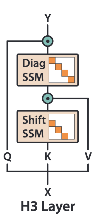
Note that while the memory mechanism on it’s own has clear computational benefits, it is also clear from subsequent adoption that it is most valuable when combined with the multiplicative interactions introduced by the H3 Block. We believe that the best interpretation of the success of this joint mechanism is indeed in terms of ‘Linear Attention’, and refer readers to the original H3 paper for more intuition.
The Shift-SSM as a Memory Mechanism
How then might one imagine implementing a mechanism to explicitly store the recent past in a recurrent architecture? One of the simplest mechanisms could be thought of as a fixed-size stack, where inputs $u_k$ are written onto the stack at each timestep, and once the stack is full, the oldest items ‘fall off’ making space for new items. In the H3 block, the authors propose to implement such a fixed-size stack explicitly within the hidden state of an SSM through a specific restricted parameterization which they call a Shift-SSM. Explicitly, this is given as: \[\begin{aligned} \mathbf{x}_{k} & = \mathbf{\bar{A}}_{\text{shift}}\mathbf{x}_{k-1} + \mathbf{\bar{B}}_{\text{shift}}u_k, \\ y_k & = \mathbf{\bar{C}}\mathbf{x}_k, \end{aligned}\]
exactly identical to a standard SSM, but crucially with the recurrent connectivity matrix (\(\mathbf{\bar{A}}\)) set to be a shift operator, and the input projection (\(\mathbf{\bar{B}}_{\text{shift}} = e_1\)) set to be the first canonical basis vector: \[\begin{aligned} \mathbf{\bar{A}}_{\text{shift}} = \begin{bmatrix} 0 & 0 & 0 & \cdots & 0 & 0 \\ 1 & 0 & 0 & \cdots & 0 & 0 \\ 0 & 1 & 0 & \cdots & 0 & 0 \\ 0 & 0 & 1 & \cdots & 0 & 0 \\ \vdots & \vdots & \vdots & \ddots & \vdots & \vdots \\ 0 & 0 & 0 & \cdots & 1 & 0 \end{bmatrix}, \quad \mathbf{\bar{B}}_{\text{shift}} = \begin{bmatrix} 1 \\ 0 \\ 0 \\ 0 \\ \vdots \\ 0 \end{bmatrix}. \end{aligned}\]
Example
If we consider the sequence \(u_0, u_1, \ldots u_T\), given an initial hidden state of \(\mathbf{x}_{-1} = \mathbf{0}\), we see that running the equations forward yields a hidden state exactly as desired: \[\mathbf{x}_{-1} = \begin{bmatrix} 0 \\ 0 \\ 0 \\ \vdots \\ 0 \end{bmatrix}, \quad \mathbf{x}_0 = \begin{bmatrix} u_0 \\ 0 \\ 0 \\ \vdots \\ 0 \end{bmatrix}, \quad \mathbf{x}_1 = \begin{bmatrix} u_1 \\ u_0 \\ 0 \\ \vdots \\ 0 \end{bmatrix}, \quad \cdots \quad\] \[\ldots \quad \mathbf{x}_{N+1} = \begin{bmatrix} u_{N+1} \\ u_{N} \\ \vdots \\ u_1 \end{bmatrix}, \quad \cdots \quad \mathbf{x}_{T} = \begin{bmatrix} u_{T} \\ u_{T-1} \\ \vdots \\ u_{T-N} \end{bmatrix}.\]
How is this a convolution?
We now approach the core confusion regarding this Shift-SSM and its adoption in later work: how is this full recurrent neural network equivalent to a small convolutional kernel applied over the sequence \(\vec{u} = \{u_t\}_{t=0}^T\)? One way to understand this is through the initial discussion of accelerating an SSM through conversion to a global convolution. However, as we will show in the next section, the implementation of this model varies significantly from the implementation of diagonal SSMs, and we believe this is not the most intutive interpretation. Instead, consider simply computing the output of the Shift-SSM, through application of the \(\bar{\mathbf{C}}\) matrix to each of the hidden states listed above. We can see that \(\mathbf{x}_t = \begin{bmatrix} u_{t-1}, & u_{t-2}, & \ldots, & u_{t-N} \end{bmatrix}^T\) at each timestep is essentially a sliding window of the past \(N\) inputs, computed a fixed size \(N\) linear projection of these inputs is effectively the same as just directly convolving \(\bar{\mathbf{C}}\) with the input sequence! In otherwords, \(\bar{\mathbf{C}}\) now becomes our convolution kernel: \[\begin{aligned} y_k & = \mathbf{\bar{C}} \mathbf{x}_t = \mathbf{\bar{C}} \cdot \begin{bmatrix} u_{t}, & u_{t-1}, & \ldots, & u_{t-N} \end{bmatrix}^T \\ & = \begin{bmatrix} \bar{C}_0 u_{t}, & \bar{C}_1 u_{t-1}, & \ldots, & \bar{C}_{N} u_{t-N} \end{bmatrix} \\ \Rightarrow \vec{y} & = \mathbf{\bar{C}} \star \vec{u} \end{aligned}\]
In practice, the hidden state \(N\) of the Shift-SSM is typically limited to only 2 to 4 elements, thereby yielding a small convolutional kernel of size 2 to 4. Thus, in the H3 work, and in all later models which adopt this architectural motif, the authors explicitly avoid implementing the full recurrence relation, opting instead to replace the full shift-SSM block with this equivalent single small convolutional layer.
Note that there are now two distinct but related types of convolution that we are discussing when talking about SSMs. One is the global convolution, which arises from ‘unrolling’ a traditional diagonal SSM and converting it into a dense convolutional kernel the same size as the input sequence. The second type, is a small local (\(N\)-element) convolutional kernel applied to the sequence length, which arises similarly from unrolling a shift-SSM (with an \(N\)-dimensional hidden state), as we describe above.
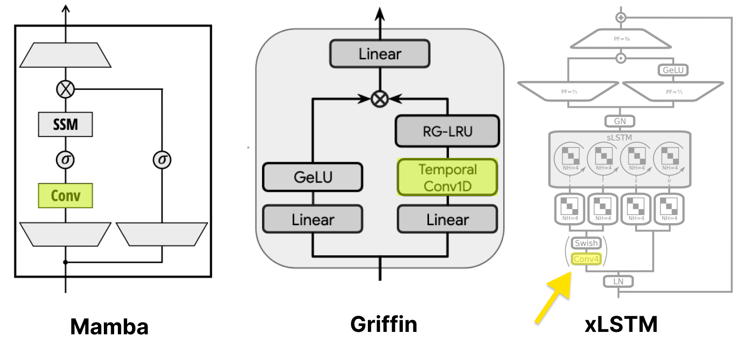
Mamba, xLSTM and Griffin
While the introduction of this block was a significant step forward for SSMs applied to language, and further allowed them to solve associative recall tasks, subsequent work has noted further limitations with these models. One of these core limitations was with respect to ‘selectively’ processing data in an input dependant manner. This led to the introduction of a number of ‘selective’ and ‘gated’ architectures including Mamba, Griffin, and xLSTM. We will not outline the details of these models, but we will highlight one core feature: the conservation of this specific small convolutional kernel (and the subsequent loss of reference to a Shift-SSM) in all of these models.
Limitations of the Convolution Parameterization
So, if the convolution is equivalent to the Shift-SSM, why is this Shift-SSM view so important that we feel the need to write an entire blog post about it? Simply put, the this equivalence only holds when \(\mathbf{A}\) is exactly the shift matrix given above, and \(\mathbf{B}\) is exactly the first canonical basis vector. The convolution parameterization of the Shift-SSM then asserts that these paramters are exactly set this way, and fixed throughout training.
In short, we argue that this limited parameterization hinders the expressivity of the model, and when understood in terms of the original goal of storing memory of the recent past in an RNN hidden state, there exist many more possibile parameterizations for such a Shift-like-SSM which no-longer are equivalent to a single small convolution layer. To exemplify this, in the following section we will highlight a recent class of recurrent neural networks built to exhibit traveling waves within their hidden state, and show how these contain the Shift-SSM above as a special case, while also providing evidence for improved performance with more flexible parameterization.
Traveling Waves and Memory
A recent line of work has aimed to study the memory storage function of wave-like dynamics in recurrent neural networks, inspired by viewpoints of physics and neuroscience. Specifically, in an ICLR 2024 paper titled “Traveling Waves Encode the Recent Past and Enhance Sequence Learning” by Keller et al., the authors aim to investigate the hypothesis that wave-dynamics are a natural mechanism for invertibly encoding a history of disturbances to a system, and therefore built simple RNN to precisely implement the one-way one-dimensional wave equation, \[\begin{equation*} \label{eqn:wave} \frac{\partial h(x, t)}{\partial t} = \nu \frac{\partial h(x, t)}{\partial x} \end{equation*}\]
where \(h(x,t)\) represents the value of the hidden state at spatial position \(x\) and time \(t\), and \(\nu\) is the associated wave velocity. When discretized over space (treating each spatial position as a separate neuron) and time (with timestep \(\Delta t\)), this wave equation yeilds the following recurrence relation: \[\begin{equation*} \label{eqn:shift} \mathbf{h}_{t+1} = \Sigma \mathbf{h}_t \hspace{5mm} \textrm{where} \hspace{5mm} \Sigma = \begin{bmatrix} 1-\nu' & \nu' & 0 & \cdots & 0\\ 0 & 1-\nu' & \nu' & \cdots & 0\\ \vdots & \vdots & \vdots & \ddots &\vdots\\ 0 & 0 & 0 & \cdots & \nu'\\ 0 & 0 & 0 & \cdots & 1-\nu'\\ \end{bmatrix} . \end{equation*}\]
where \(\nu' = \nu \Delta t\). In their paper, the authors argue that this recurrence can be seen to be equivalent to a convolution over the hidden state with a small convolutional kernel \(\mathbf{a} = \left[0, 1-\nu, \nu\right]\). In otherwords, showing following equivalence: \(\mathbf{a} \star \mathbf{h}_{t-1} = \Sigma \mathbf{h}_{t-1}\). They then build a simple RNN architecture using this convolutional recurrence and a ReLU non-linearity \(\sigma\): \[\begin{equation*} \label{eqn:wrnn} \mathbf{h}_{t+1} = \sigma (\mathbf{a} \star \mathbf{h}_t + \mathbf{B} \mathbf{u}_t + \mathbf{b}) \end{equation*}\]
The authors demonstrate that such a wave-based RNN dramatically outperforms other wave-free RNN architectures on tasks which require long-sequence memory such as copy tasks, and sequential image classification tasks. Given that recent work has shown that state space models such as Mamba are very bad at performing copy tasks (Jelassi et al.), it is then interesting to consider the relationship between these SSMs and such a simple wave-RNN.
Waves in Mamba
In fact, if we look carefully, we can see that for a wave speed of \(\nu'=1\), the \(\Sigma\) matrix of the wave-RNN is exactly equivalent to the \(\mathbf{\bar{A}}_{\text{shift}}\) of the Shift-SSM. Furthermore, if \(\sigma\) is set to the identity, and \(\mathbf{B} = e_1\) then we exactly recover the full Shift-SSM (and indeed in the wave-RNN model, the authors do initalize \(\mathbf{B} = e_1\)). What does this equivalence mean?
One interpretation of this equivalanence is that state space models such as Mamba, Griffin, and xLSTM already implicitly have waves of activation propagating within their hidden states. These waves propagate over the small 4-dimensional hidden state of an implicit shift-SSM.
To demonstrate this visually, in the following, we plot what these waves look like if we replace the convolutional form of the Shift-SSM from the original Mamba repo, with a full shift-matrix recurrence. Explicitly, from the original Mamba repo the shift-SSM is implemented as:
x = self.act(self.conv1d(x)[..., :seqlen])
In order to access the hidden state, we instead propose to replace this conv1d layer with a full Shift-SSM implemented as:
class Shift_RNN_Cell(nn.Module):
    def __init__(self, n_inp, n_hid, n_ch=1, ksize=3):
        super(Shift_RNN_Cell, self).__init__()
        self.n_hid = n_hid
        self.n_ch = n_ch
        self.Wx = nn.Linear(n_inp, n_hid * n_ch)
        self.Wy = nn.Conv1d(n_ch, n_ch, ksize,
                          padding=ksize//2,
                          padding_mode='zeros',
                          bias=False)
        self.act = nn.Identity()

        # Initialize Read-in weights (B matrix) to be the first canonical basis vector
        nn.init.zeros_(self.Wx.weight)
        nn.init.zeros_(self.Wx.bias)
        with torch.no_grad():
            w = self.Wx.weight.view(n_ch, n_hid, n_inp)
            w[:, -1] = torch.eye(n_ch, device=device)
        # Freeze the read-in weights
        for param in self.Wx.parameters():
            param.requires_grad = False

        # initalize convolution to be shift matrix
        with torch.no_grad():
            wts = torch.zeros(n_ch, n_ch, ksize)
            nn.init.dirac_(wts)
            wts = torch.roll(wts, 1, -1)
            self.Wy.weight.copy_(wts)
        # Freeze the recurrent weights
        for param in self.Wy.parameters():
            param.requires_grad = False

    def forward(self,x,hy):
        hy = self.act(self.Wx(x) + self.Wy(hy.view(-1, self.n_ch, self.n_hid)).flatten(start_dim=1))
        return hy


class Shift_SSM(nn.Module):
    def __init__(self, n_inp, n_hid, n_out, n_ch=1, ksize=3):
        super(wRNN, self).__init__()
        self.n_hid = n_hid
        self.n_ch = n_ch
        self.cell = Shift_RNN_Cell(n_inp, n_hid, n_ch, ksize)
        self.readout = nn.Linear(self.n_hid, n_out)

    def forward(self, x):
        ## initialize hidden states
        hy = Variable(torch.zeros(x.size(0), self.n_ch * self.n_hid)).to(device) # (B, D * W)
        self.y_seq = torch.zeros((*hy.shape, x.shape[-1]), device=device)
        out_seq = torch.zeros(x.shape, device=device)

        for t in range(x.shape[-1]):
            hy = self.cell(x[t], hy)

            output = ((self.readout.weight * hy.view(x.shape[0], self.n_ch, self.n_hid)).sum(-1)
                      + self.readout.bias)
            out_seq[t] = output

        return output, out_seq
Doing this for the original Mamba architecture, we get the following visualization of the hidden state (vertical axis) over timesteps (horizontal axis), while the model processes a sequence of length 225. We see from the diagonal bands of activity that indeed, there are waves of activation propagating over the small 4-dimensional hidden state.
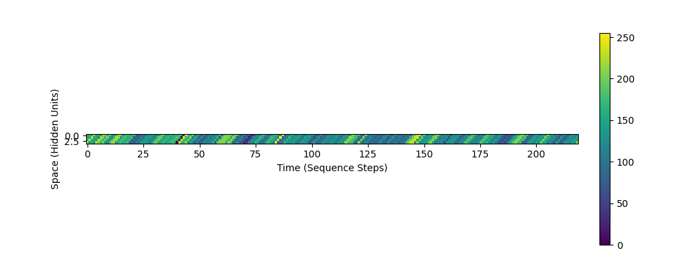
To increase the visibility of these waves, we can also increase the size of the hidden state of the Shift-SSM (equivalent to the size of the conv1d kernel used before). Below we show what these waves look like for a 16-dimensional hidden state:
From this simple re-interpretation and re-implementation, we immediately see other possible modifications that can be made to Mamba to potentially improve the memory storage performance, analagous to the explorations performed for wave-based recurrent neural networks. For example, we could use the variable velocity wave formulation of the wave-RNN, with a flexible parameter $\nu$ instead of assuming $\nu=1$. Doing so yields a ‘Shift-like-SSM’ state with the following dynamics:
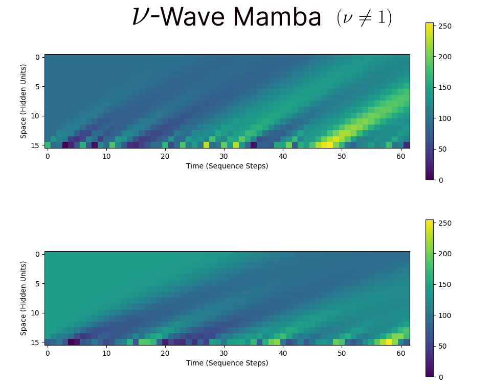
Ultimately, we see that this is not an exact shift, this has significantly more complex dynamics, and could allow for greater memory storage with such a simple mechanism.
Limitations: Computational Efficiency
While we see that this increased flexibility of parameterization can yield more complex hidden state dynamics, and thereby potentially improve the memory performance of these models (as has been achieved for simple-RNNs), this performance also comes with the cost of additional computational complexity which must again be accounted for. While we do not provide explicit methods for accelerating arbitrary wave-recurrence relations in this post, we note that many such cases are ammenable to the same acceleration techniques used for traditional SSMs (the unrolled-convolution formulation, diagonalization, and the parallel associative scan). Thus, while in the current above implementation there will be a significant computational cost to using the explicit shift-SSM, we do not believe this is a fundamental limitation in the long run.
Conclusion
In conclusion, in this blog post we have aimed to highlight the importance of the specific small convolution layer in modern state space model architectures, and give intuition for why such a layer has been conserved across all state-of-the-art models. We have shown that it can be interpreted using ideas of wave-dynamics, opening up new avenues for potential improvements to the memory capabilities of such models.